Contributory Value

This article is featured in the 2024 edition of the Appraisal Buzz Magazine. Some other features we have in our magazine include Buzztoon comics, as well as crazy stories from appraisers and readers like you! Read all these articles and more in the latest edition HERE. If you want to make sure you are receiving the print version of the Appraisal Buzz magazine in your mailbox, sign up HERE.

The sales comparison grid is where appraisers report the contributory value of differences between the subject and comparables.   

The differences are categorized by units of comparison. Gross living area (GLA), baths, and garage stalls are examples. Other units of comparison are location, site, view, quality, and condition. Stick with me: I’ll explain a strategy to develop market-based adjustments throughout the grid.

This quote from page 372 of The Appraisal of Real Estate 15th Edition will get us off to a good start: “Paired data and grouped data analysis are variants of sensitivity analysis, which is a method used to isolate the effect of individual variables of value.” 

This sentence is loaded with meaning. Sensitivity analysis is an umbrella term for paired data and grouped data. The idea is to use these methods to isolate the effect of individual variables on value. They operate within a model we call the sales comparison grid (SCA). The SCA is a model used to predict a value. The SCA grid includes units of comparison that are imposed upon the analyst.   

Multivariable regression (MVR) is another valuation model that gets a lot of attention. It’s ideal for AVMs, mass appraisal and portfolio analysis. There’s an important difference between the MVR model and the SCA: MVR mathematically chooses the variables that work best to predict value. Baths, bedrooms, and GLA may be combined to represent house capacity. This effect is called multicollinearity. Multicollinearity is an advantage for MVR but is hazardous in the SCA.

Please, PLEASE resist the temptation to pry a coefficient (adjustment rate) from an MVR model and cram it into your sales grid. An MVR model is all or nothing. Competency is compromised by combining MVR coefficients that “look good” with other methods in the SCA.

Back to a strategy for isolating the effect of individual variables on value: This is counterintuitive, but let’s start with the cost approach. We’ll use the analytics of the cost approach to show the contributory value of the building and to support our assertions of effective age and remaining economic life. 

Check this out from USPAP Standard Rule 1-3: “An appraiser must avoid making an unsupported assumption or premise about market area trends, effective age, and remaining life.”

Most appraisers are on board with supporting market area trends, but in my experience, few pay attention to remaining economic life. Here’s why they should: Remaining economic life divided by economic life is the percentage of cost paid by the market.   This truth will get you halfway through the grid if you handle cost data properly.

Cost data is published as average cost per foot. As the GLA increases, the total cost of GLA increases but the average cost per foot decreases. Consider this example:

If the remaining economic life is extracted from the market at 42 years, and economic life is 60 years, 42/60 = 70% of cost is market value. When marginal cost is $100, and market reaction is 70% of cost, a market-supported GLA adjustment is $70.   

Did you notice the similarity with paired sales? The cost of 200 square feet is $20,000, but the market does not pay 100% of cost. If the remaining economic life is 70% of cost, it pays $14,000; $14,000 divided by 200 square feet is $70 per square foot.

A bath adjustment can be done in a similar way. If the cost of a bath at the time of construction is $12,000, and the market pays 70% of cost, then a market-supported adjustment for a bath difference is $8,400.

This method is known as depreciated cost. But the concept is contributory value, which I’ve included in the title of this article.

Look at this example of the cost approach with site value, GLA, site improvements and indicated value by cost approach: 

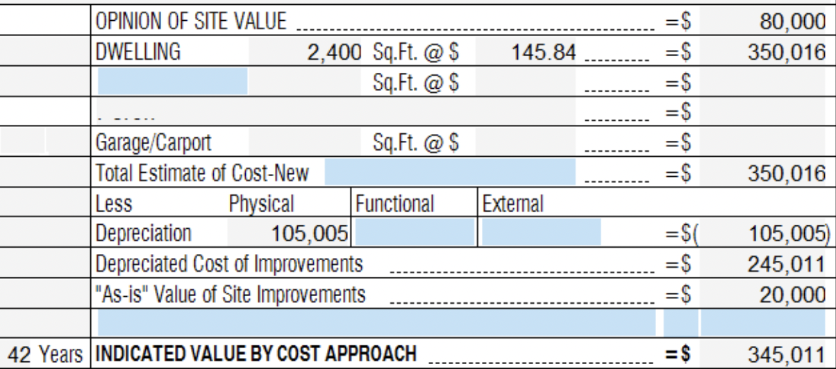
Depreciated cost of improvements is $245,000. This is what the market pays for the GLA — it’s the contributory value of the house. Total estimate of cost new is $350,000.   The remaining economic life is 42 years, so the market is paying 70% of cost. 70% of $350,000 is $245,000. Think of 70% as %CV for percentage contributory value.

Immediate benefits include:

Cost data isolates units of comparison. While MVR may combine baths with GLA, cost data always fits the sales grid and avoids multicollinearity. 

Cost data is clean. Begin your analysis without worrying about MVR built upon inconsistent MLS data. 

It’s fast. Use a web application or create your own spreadsheet to build a cost approach and crunch the numbers.

It’s easy to explain. A litigation specialist in Colorado said, “I have a much easier time explaining cost and depreciation in the courtroom than multivariable regression.”   Everyone understands 70 cents on the dollar.

Multivariable regression is a valuable tool used across the spectrum of scientific inquiry.   It works well for the valuation of groups of houses. In my experience, the total value of a group of 30 houses was predicted within 1% of the actual sale prices. The range of predicted values of individual houses was more like +/-10%. This is why AVMs are inferior to the sales comparison approach (SCA) for individual houses.

The SCA is a model that requires isolation of individual units of comparison. In my experience, there is no better way to solve half the grid than depreciated cost. When depreciated cost adjustments are applied in the grid, along with cash equivalency and market to -to-market adjustments, the result is adjusted sale prices at the bottom of the grid.   

Now the fun begins. Use adjusted pairs and sensitivity analysis to complete the analysis with confidence. Remember, “Paired data and grouped data analysis are variants of sensitivity analysis, which is a method to isolate the effect of individual variables of value.”