What Poetry and Data Analysis Have in Common
We will call this place our home.
The dirt in which our roots may grow
Though the storms will push and pull
We will call this place our home.
We’ll tell our stories on these walls.
Every year, measure how tall
And just like a work of art
We’ll tell our stories on these walls.
–Verses 1 and 2 of “North”, by Sleeping At Last
They may seem worlds apart, but poetry and market analysis have something in common. Often poetry has a meter, which can be described as the pattern and emphasis which give the lines a structure. If you read aloud the song lyrics above, you’ll hear the meter in your own voice. Add music, and it becomes even clearer.
Meter endows stanzas with lyrical patterns and meaningful emphasis, turning words into poetry. Metric derives from the same word as “meter,” and for good reason. By applying appropriate metrics an analyst can find patterns and draw conclusions about meaning in a set of data.
For our purposes you can think of metrics as comparative units of measurement used to quantify and evaluate economic activities.
For example, if an observes that larger homes sell for higher prices than smaller homes, considering price change relative to change in gross living area (GLA) is an appropriate metric to consider. The resulting marginal rate for each additional square foot of GLA is one of the most common uses of metrics found in residential appraisal. Applying this metric to marginal changes in GLA between two properties enables the appraiser to predict the corresponding change in price.
“Appropriate” is a key consideration in metrics (and meter). Applying the wrong meter can render otherwise beautiful lyrics abrasive and unintelligible. Similarly, if an appraiser applies no metric, or an inappropriate metric, the same thing can happen — data can become unintelligible and difficult to interpret, and the meaning imputed to that data could be misleading.
Case Study
Gather and organize the data.
Let’s look at an example. For this case, the subject property has a golf course view, and we’re analyzing the data below to understand the premium price we anticipate for that view. Properties with a golf course view are denoted with a “1” and those without views are denoted with a “0.” (These “dummy variables” can be useful in analysis.)
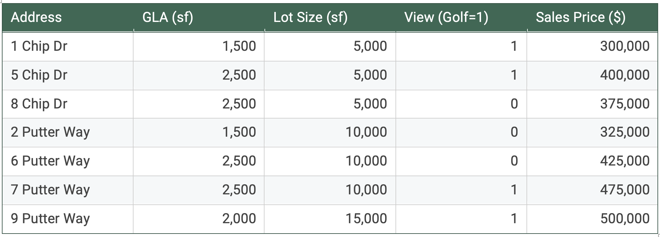
One example of applying no metric at all might be simply comparing averages (essentially a grouped pair). The average home with a golf course view sold for $418,750. The average home without a view sold for $375,000, so the golf course view premium must be $43,750, correct?
Not exactly. If we look at the pairing of 6 Putter Way with 7 Putter Way, the difference is $50,000, but the pair of 5 Chip Drive and 8 Chip Drive has a difference of only $25,000.
Maybe there’s a pattern to the golf course premium, but we can’t see it clearly just yet.
Let me pause to point out that the data above has a specific pattern by design. Real estate markets are complex, but they do have discernible patterns, because the actions of buyers and sellers are not random. While there will always be variation and irrationality in human behavior, we can generalize to a degree: A group of buyers may differ on the specific value they might place on a golf course view, but they’ll likely agree that the view is a premium. They’ll also likely agree on some factors which might influence how much that premium might be. Keep that in mind as we continue our discussion.
So, if we want to zero in on this pattern with more precision, let’s stary by applying some metrics. Not just any metric will do. If we apply the wrong one, our conclusions won’t be useful; or worse, they could be misleading.
When choosing a metric, we want one that will help us discover how one thing changes relative to a change in something else. In other words, we’re looking for an independent variable that best explains the change in the dependent variable.
Isolate the variable.
The first step is to isolate the variable we are studying. One method to do this is modeling.
In modeling, we apply a known or hypothetical pattern for one part of the data, to better study another part. (Appraisers know this process well — we use the term “adjustments.”) In this case, let’s assume some modeling factors which will best isolate the variable of view. If we look at the grid, we see independent variables of GLA, lot size, and view.
Let’s assume that differences in GLA and lot size are a known quantity. Differences in GLA we will model (adjust) at $100/sf, and differences in lot size (surplus land) we will model at $10/sf. In the grid below, I’ve added a column called “Modeled Price.” This column adjusts every sale for differences in GLA and lot size making them equivalent to a property with 1500 sf and a 5000 sf lot. (You could just as easily apply the modeling factors to any other GLA and lot size.) This isolates the variable of view and allows us to see the golf course premium, which is in the last column.
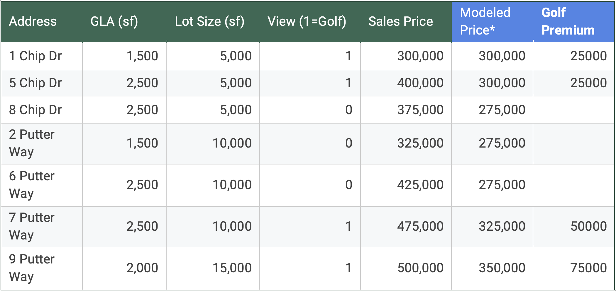
*The modeled price is the price which would result if every sale were adjusted for GLA and lot size.
Now that we’ve isolated the golf course premium, we can see that it varies from $25,000 to $75,000. So, the question then becomes: Why? Why is the golf course premium not consistent? Metrics can help answer that question.
We have a couple of potential metrics, GLA and lot size. The way that we apply the metric is to divide the golf course premium by the potential metric. Let’s consider GLA first.

The last column shows the associated golf course premium per square foot of GLA. The result is a wide range: from $10/sf to $38/sf. When we see that our GLA ranges from 1500 sf to 2500 sf, that would mean that applying the “premium per GLA” metric yields a range of premiums from $15,000 to $95,000. That’s wider than our range with no metric at all! This is an example of how the wrong metric can be worse than no metric at all.
So, GLA wasn’t a good metric. What about lot size? Let’s perform the exact same calculation, but instead of dividing the golf premium by GLA, we’ll divide it by lot size.
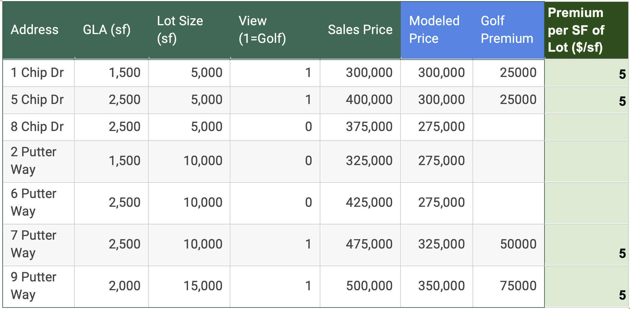
When we look at the lot size as our metric, the golf course premium finally makes sense: it’s highly correlated with lot size. In this case, 100% of the data supports the conclusion that the best predictor of the golf course premium is the lot size. The “premium per sf of lot” metric of $5/sf of the lot size will predict the observed golf course premium for every observation in our data set.
Apply the metric.
Now let’s pretend that 1 Chip Drive is the subject property. We’ll select 3 sales from the data set for comparison and make an adjustment for the subject’s golf course premium without considering any metric. If we apply the grouped pair conclusion of $43,750, which we referenced earlier, the grid would look like this:
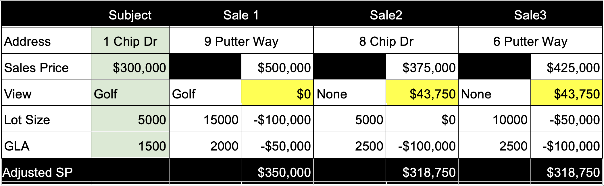
The average adjusted sales price is approximately $329,000, which is nearly 10% higher than the sales price, so this technique when applied to these sales resulted in a poor predictor of the $300,000 price. Without the appropriate metric, any combination of sales will result in a potential value conclusion which is a poor predictor of value. (Remember, the Fannie Mae definition of market value begins with “the most probable price.”)
Now, let’s look at the grid with the appropriate metric applied:
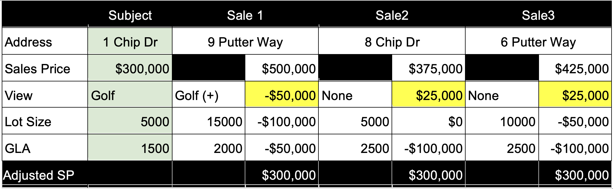
It’s possible this grid looks a little different than you anticipated. In order to apply the metric properly, you have to consider the source of the premium. Even though the lot size for sales 2 and 3 differed, the golf course premium did not. That’s because the premium is tied to the lot size of the property. So the adjustment calculation is the difference in view premium for each sale.
This is a case where it’s helpful to consider the dummy variable (0 or 1 to denote view) when calculating view:
$5 x LOT SIZE x VIEW = PREMIUM
Therefore, the calculation for the premiums for the subject and comparables would look like this:
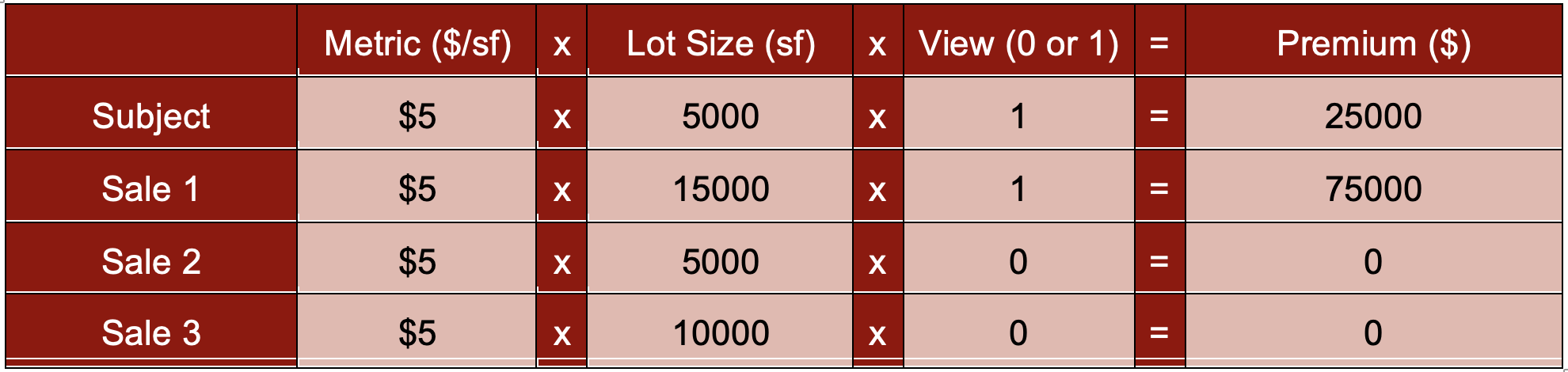
The adjustments applied are, therefore, the differences between the premiums. For comparables without a golf course view, any lot size will still result in a $0 premium, since multiplying anything by zero will equal zero. While it’s completely logical, it may not be immediately intuitive.
You may notice that you could also look at this data set from a different perspective: What if we kept the golf course premium static (not a variable number) and instead considered the contributory value of the lot to vary as a function of whether it had a golf course view? You could indeed, so the question becomes, which is the “right” way?
In this case study, you could do either one and get the same result. But chances are, you’ll consider one way more intuitive, faster to calculate, and easier to explain.
Beyond Case Studies
Of course, real world data sets are much more complicated. That makes it even more difficult to apply appropriate metrics, but also that much more necessary.
At first, it may not be immediately apparent what the best metric might be for the property characteristic you’re trying to understand, but here’s a simple roadmap:
Begin with logic.
In our case study, it’s fairly intuitive that larger lots might carry a higher premium. Larger lots likely have a wider field of view, more frontage on the golf course, and potentially more backyard space or more windows from which to enjoy the view.
Consider the cost.
If considering an improvement, look at what variables influence the cost of that amenity.
Look for complements and corollaries.
Your powers of observation will often help identify complementary property characteristics which may influence value. For instance, is there a correlation between the number of bedrooms and the value of additional bathrooms? You might notice that when there are only 3 bedrooms, a 4th full bathroom doesn’t add as much value.
Experiment with your data.
Finding ways to export data into tables allows you to sort, filter, and calculate a wide variety of metrics quickly, so you can let the data speak for itself.
Don’t reinvent the wheel.
When you notice metrics that make sense, track those and calculate them automatically. You don’t have to start from scratch every time! Remember, human behavior is predictable — not perfectly so, but still predictable.
In my practice, I apply metrics regularly in researching and applying adjustments in the sales comparison approach. I regularly use various metrics to apply adjustments for location, view, quality, age, condition, room count, and several amenities. Once you expand your mindset to considering metrics, your appraisals will become more accurate, and your analysis will become more efficient, resulting in a better appraisal in less time.
Share this article
Written by : Brent Bowen
Brent is the president of Texas Valuation Professionals, Inc. (www.txvaluepro.com) in Plano, Texas and has been appraising residential real estate in north Texas for 25 years. He graduated from Baylor University with an enthusiasm for both economics and real estate, which made real estate appraisal a perfect fit. Rarely satisfied with the status quo, Brent hopes to always be open to further development, both professionally and personally.